Thermal conductivity of three phase structure

For details about the effective thermal conductivity calculation, please see here.

Overview

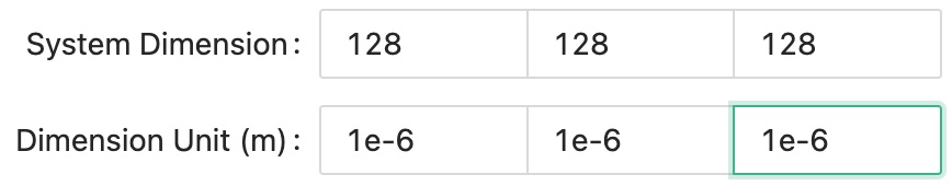
First, we will setup a cubic simulation with 128 microns along each dimension, that is 128 simulation grids times 1 micrometer for each grid.

Next, we will add three phases into the system, one for the matrix phase, another for the slab with higher conductivity, and the other for the embedded particle with lower conductivity.

Lastly, we will setup a structure with slab and random ellipsoid for the composite material.

Step 1: Fill Input

Follow the introduction to the input part in the user manual and make sure you fill all of the blank boxes in the following four sections.

Dimension

Output

Choose vti for the output format, since we may want to visualize with Paraview.

System

Choose "Thermal" system for the System Type. Besides from the effective properties of thermal conductivity, we also want to calculate a field distribution under external applied thermal gradient, so we need to turn on the Distribution switch and set an Tenp. grad (k/m) value, the temperature gradient in kelvin per meter.

Next, set the reference thermal conductivity value to be used in our solver.

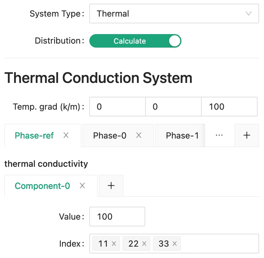
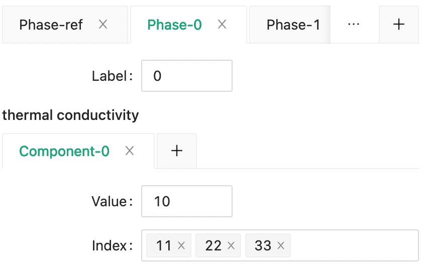
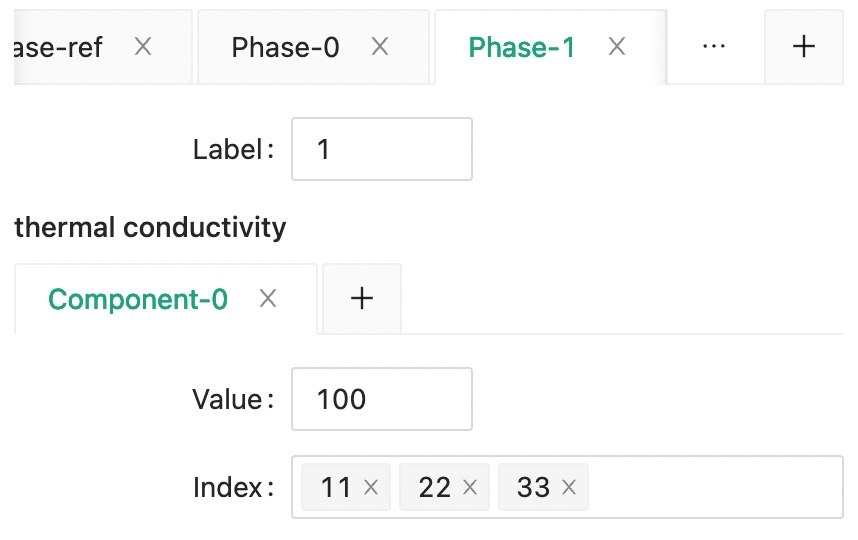
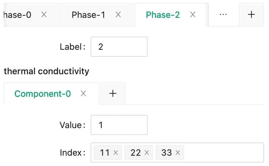
Then, set the thermal conductivity for the three phases.

Structure

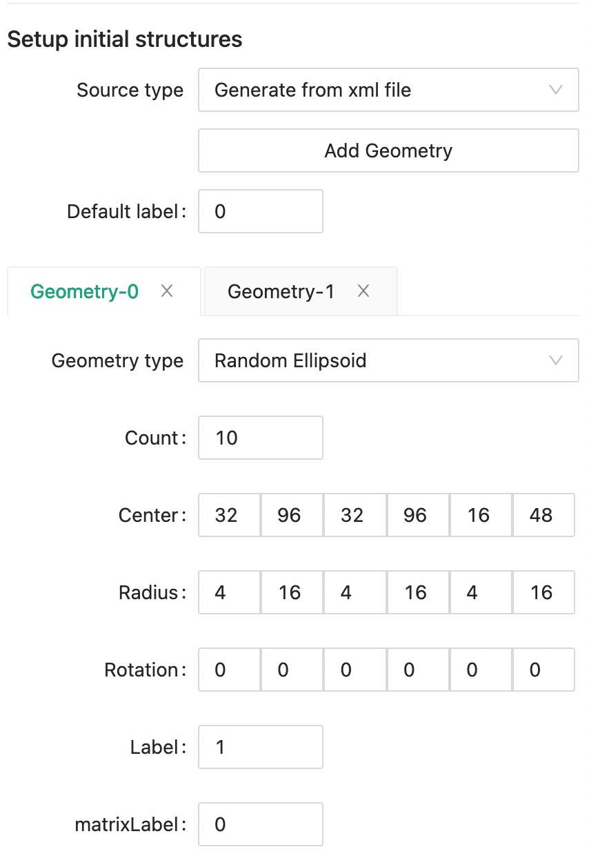
Since we want to generate the structure within the effective properties simulation program, we should choose "Generate from xml file" for the Source type.

Click Add Geometry button to create a new geometry tab, and set label 0 as the Default label.

We want to create 10 randomly generated ellipsoids whose centers are located in the lower half of the 128 cube, and leave the upper half for the slab.

The ellipsoid radius is random value between 4 to 16 grid points, and there is no rotation added to the ellipsoid.

We will assign phase label 1 to this newly defined geometry and set its matrix label to be phase 0.

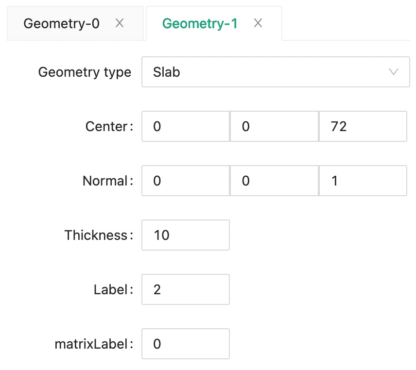
To set the slab structure, we click the Add Geometry again and choose Slab for Geometry type

Step 1.5: Or Import Input

If you don't want to enter all of the values manually, you may import the following input file directly into the software.

Save the following content into a local file, then click the File -> Import in the menu to read your saved file.

<input>
  <dimension>
    <nx>128</nx>
    <ny>128</ny>
    <nz>128</nz>
    <dx>1e-6</dx>
    <dy>1e-6</dy>
    <dz>1e-6</dz>
  </dimension>
  <output>
    <format>vti</format>
  </output>
  <system>
    <type>thermal</type>
    <distribution>1</distribution>
    <external>
      <temperatureGradient>
        <x>0</x>
        <y>0</y>
        <z>100</z>
      </temperatureGradient>
    </external>
    <solver>
      <ref>
        <tensor>
          <name>thermal_conductivity</name>
          <rank>2</rank>
          <pointGroup>custom</pointGroup>
          <component>
            <value>100</value>
            <index>11</index>
            <index>22</index>
            <index>33</index>
          </component>
        </tensor>
      </ref>
    </solver>
    <material>
      <phase>
        <label>0</label>
        <tensor>
          <name>thermal_conductivity</name>
          <rank>2</rank>
          <pointGroup>custom</pointGroup>
          <component>
            <value>10</value>
            <index>11</index>
            <index>22</index>
            <index>33</index>
          </component>
        </tensor>
      </phase>
      <phase>
        <label>1</label>
        <tensor>
          <name>thermal_conductivity</name>
          <rank>2</rank>
          <pointGroup>custom</pointGroup>
          <component>
            <value>100</value>
            <index>11</index>
            <index>22</index>
            <index>33</index>
          </component>
        </tensor>
      </phase>
      <phase>
        <label>2</label>
        <tensor>
          <name>thermal_conductivity</name>
          <rank>2</rank>
          <pointGroup>custom</pointGroup>
          <component>
            <value>1</value>
            <index>11</index>
            <index>22</index>
            <index>33</index>
          </component>
        </tensor>
      </phase>
    </material>
  </system>
  <structure>
    <matrixLabel>0</matrixLabel>
    <sourceType>xml</sourceType>
    <geometry>
      <type>ellipsoid_random</type>
      <count>10</count>
      <centerXMin>32</centerXMin>
      <centerXMax>96</centerXMax>
      <centerYMin>32</centerYMin>
      <centerYMax>96</centerYMax>
      <centerZMin>16</centerZMin>
      <centerZMax>48</centerZMax>
      <radiusXMin>4</radiusXMin>
      <radiusXMax>16</radiusXMax>
      <radiusYMin>4</radiusYMin>
      <radiusYMax>16</radiusYMax>
      <radiusZMin>4</radiusZMin>
      <radiusZMax>16</radiusZMax>
      <rotationXMin>0</rotationXMin>
      <rotationXMax>0</rotationXMax>
      <rotationYMin>0</rotationYMin>
      <rotationYMax>0</rotationYMax>
      <rotationZMin>0</rotationZMin>
      <rotationZMax>0</rotationZMax>
      <label>1</label>
      <matrixLabel>0</matrixLabel>
    </geometry>
    <geometry>
      <type>slab</type>
      <centerX>0</centerX>
      <centerY>0</centerY>
      <centerZ>72</centerZ>
      <normalX>0</normalX>
      <normalY>0</normalY>
      <normalZ>1</normalZ>
      <thickness>10</thickness>
      <label>2</label>
      <matrixLabel>0</matrixLabel>
    </geometry>
  </structure>
</input>

1
2
3
4
5
6
7
8
9
10
11
12
13
14
15
16
17
18
19
20
21
22
23
24
25
26
27
28
29
30
31
32
33
34
35
36
37
38
39
40
41
42
43
44
45
46
47
48
49
50
51
52
53
54
55
56
57
58
59
60
61
62
63
64
65
66
67
68
69
70
71
72
73
74
75
76
77
78
79
80
81
82
83
84
85
86
87
88
89
90
91
92
93
94
95
96
97
98
99
100
101
102
103
104
105
106
107
108
109
110
111
112
113
114
115
116
117
118
119
120
121
122
123

Step 2: Export Input

Click the Create Inputs button. Select the folder that you want to run the simulation in, and create a file named input.xml.

This step is simple but very important because the input.xml file is a prerequisite for starting any calculation.

Step 3: Run calculation

Make sure you have finished Step 2, you have to click the Create Input button, because it will both export the input.xml file and set the current working directory to that folder.

Then, you can click the Start simulation button to start the calculation. If you have not click the Create Input button and create the input.xml file, nothing will happen because the program does not know where to look for the input.xml file.

Step 4: Check Output

You will see the following output files in your simulation folder. Meaning for each of the files are explained in the Dielectric System.

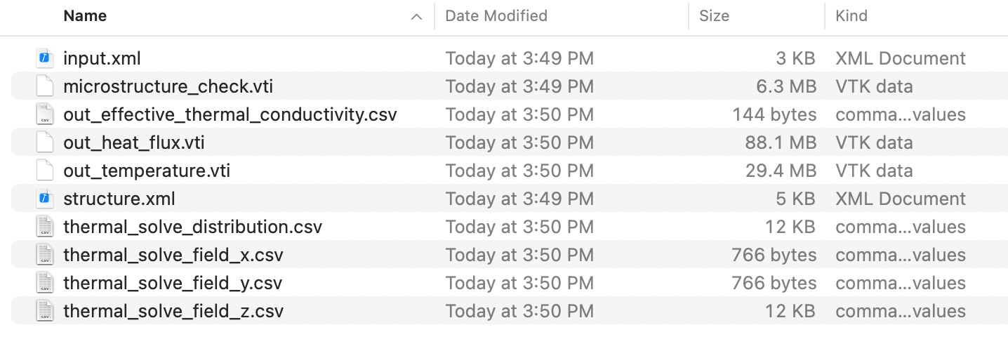
Overall, there are two types of output data, vti files for 3D data, and csv files for tabular data.

Step 4.1: Check 3D data

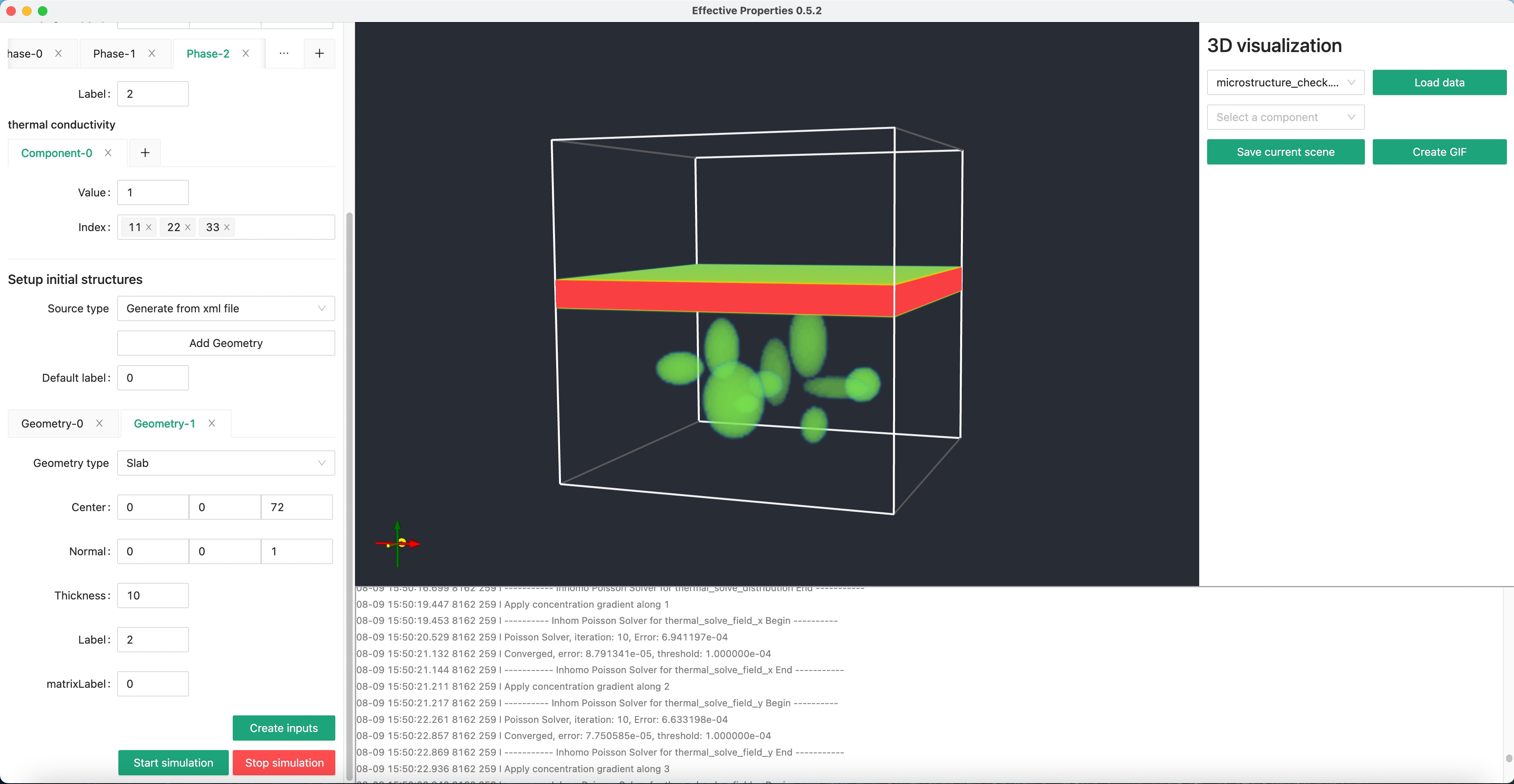
Within our software, you can quickly check a 3D vti data file.

Select the file you want to visualize using the dropdown menu, then click Load data button.

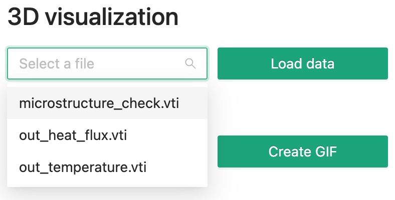
Then you will see something like this.

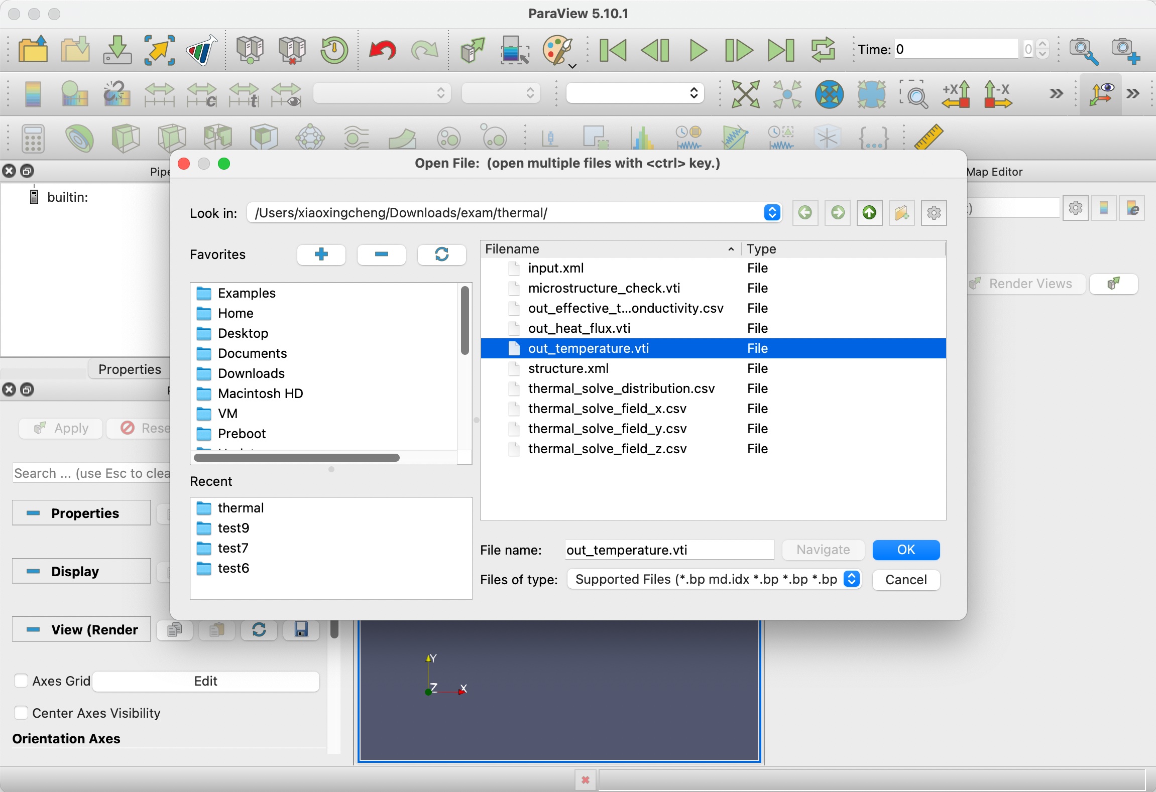
Step 4.2: Paraview

Next, we can try visualizing other files with Paraview. Click the first Open icon in the tool bar.

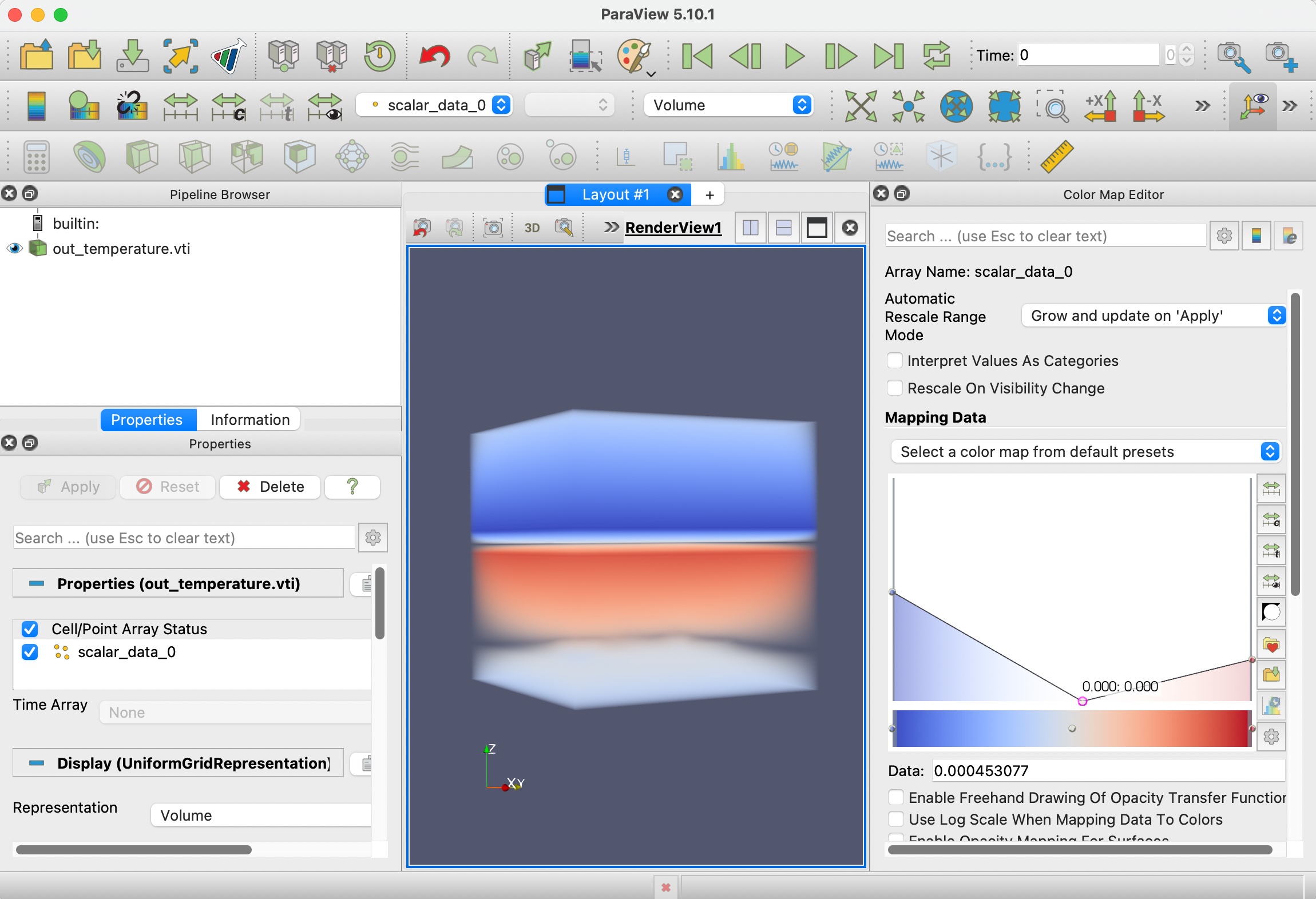
After the data is loaded, click Apply, then switch to Volume rendering and choose scalar_data_2, which is electric field along z for visualization.

We also need to tune the color lookup table to add some transparency to the data.

Step 4.3: Check tabular data

Though 3D data looks cool, the more important thing probably is still the effective permittivity, out_effective_permittivity.csv.

Index	1	2	3
1	+9.580886e+00	+1.757357e-03	-4.381574e-03
2	+1.757357e-03	+9.566548e+00	+1.616383e-03
3	-9.079212e-03	+3.559258e-03	+6.093892e+00

Thermal conductivity of three phase structure #

Overview #

Step 1: Fill Input #

Dimension #

Output #

System #

Structure #

Step 1.5: Or Import Input #

Step 2: Export Input #

Step 3: Run calculation #

Step 4: Check Output #

Step 4.1: Check 3D data #

Step 4.2: Paraview #

Step 4.3: Check tabular data #